Enclave Cryptography: GRECO for FHE + ZK Consistency

Interest in Fully Homomorphic Encryption (FHE) has been growing rapidly, and with it, more mature applications are emerging that combine it with zero-knowledge proofs (ZKPs) or multi-party computation (MPC). These hybrid systems unlock powerful new use cases, but they also bring fresh challenges that require clever cryptographic engineering.

Imagine that a major city has six large-scale hospitals. In order to predict and rapidly respond to emergent epidemics, the hospitals would like to know the aggregate number of patients treated for a variety of common contagions each week. However, for competitive reasons, the hospitals do not wish to divulge their individual numbers with one another.

Using a threshold FHE scheme, each of the hospitals can encrypt their numbers to a key controlled by a committee trusted by the group of hospitals, such that they have strong guarantees that only the aggregate output will be decrypted.

But if the program can't see the inputs, how can it validate that the inputs are correct?

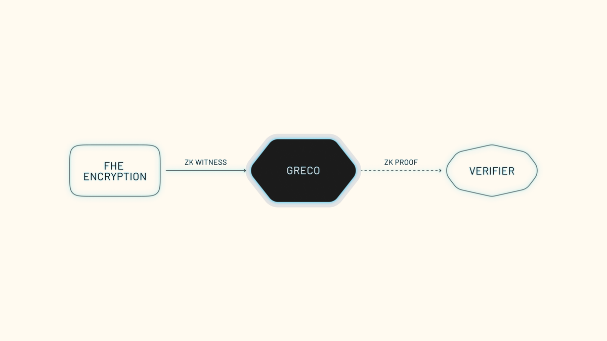
That’s where GRECO [Bot24], a zero-knowledge proof of correct encryption, comes in. It lets anyone verify that a ciphertext is correctly encrypted under the right FHE key without revealing the plaintext. Together with the application-level checks, GRECO guarantees that the plaintext satisfies the required validity constraints (for example, being within the allowed domain or matching the expected structure) and that it is encrypted with the correct FHE key.

In practice, constructions like GRECO become an essential integrity check whenever multiple parties contribute encrypted inputs to a shared computation (cheating as a single party would only wreck their own results). Systems such as Enclave, which execute confidential multi-party computation across untrusted participants, rely on mechanisms like GRECO to ensure that each encrypted input is both valid and correctly bound to the value being proven.

Let's unpack how GRECO works.

Under the Hood

In this article, like in the original paper, we will focus on BFV and SNARKs, assuming the reader already has a basic grasp of both. You don’t need to know all the math, just the core ideas. For anyone interested in going deeper, see this great article on FHE by Jeremy Kun and this other article on SNARKs by Vitalik Buterin.

Rather than inventing new primitives, GRECO extends ideas from FHE and ZKPs, relying on the Residue Number System (RNS) and optimized polynomial evaluation to make the math line up properly.

What to Prove

Before diving deeper, we first need to understand what we actually want to prove in zero knowledge: the equation that convinces the verifier that a ciphertext is the result of the correct encryption of a plaintext. To do that, let’s recall how encryption works in BFV.

Given a public key $pk = (p_0, p_1)$ and a plaintext $m$, the ciphertext $(c_0, c_1)$ is computed as:

$$ \begin{aligned} u &\leftarrow R_2, \quad e_1, e_2 \leftarrow \chi \\ c_0 &= pk_0 \cdot u + e_1 + \Delta \cdot m \\ c_1 &= pk_1 \cdot u + e_2 \end{aligned} $$

Here $u$ is a random binary polynomial, $e_1$ and $e_2$ are error terms sampled from a noise distribution $\chi$, and $\Delta = \lfloor q / t \rfloor$ is a scaling factor that maps the plaintext space $t$ into the ciphertext modulus $q$.

This simple pair of equations hides a lot of cryptographic machinery, but for now all we need to remember is that the ciphertext is a noisy linear combination of the public key and the plaintext, carefully balanced so that only the secret key can recover $m$. Solving a linear combination is easy, but once you add noise, the problem becomes NP-hard, forming the basis of the Learning With Errors (LWE) assumption that modern lattice cryptography relies on.

In our zero knowledge setting, the ciphertext $(c_0, c_1)$ and the public key $(p_0, p_1)$ will act as public inputs to the proof, while the plaintext and the noise terms $(u, e_1, e_2)$ remain private witnesses.

The ultimate goal of the proof is to convince the verifier that these public values satisfy the encryption equation above, meaning the ciphertext was generated with the right public key.

Challenges

If you’ve seen RLWE before, you already know that these polynomials live in a ring modulo both $q$ and $X^N + 1$. In simple terms, $q$ keeps the coefficients bounded, meaning every number wraps around once it reaches $q$, while $X^N + 1$ keeps the degree bounded, making polynomial multiplication wrap neatly back on itself. Together, they form the space $R_q = Z_q[X] / (X^N + 1)$.

Now, there are two main challenges that make proving this equation inside a ZK circuit tricky:

• Depending on the configuration, $q$ can be much larger than $p$ (the modulus defining the SNARK field).
• On top of that, solving this equation directly with $R_q$ and all the operations would be far too expensive in a zero knowledge context.

This is exactly where GRECO steps in. It introduces a way to express the ciphertext–plaintext relationship without having to reproduce all the complex arithmetic that happens over the $q$-modulus ring inside the proof system. In other words, GRECO bridges the world of FHE (which lives in $R_q$) with that of SNARKs (which operate in a field modulo $p$), keeping the proof lightweight while preserving full correctness.

Splitting the Modulus with RNS

The solution to keep the modulus $q$ from exceeding $p$ comes from a technique already used in many RLWE-based schemes: the Residue Number System (RNS), which is built on the Chinese Remainder Theorem (CRT).

In short, instead of working with one large modulus $q$, we split it into several smaller moduli $q_i$. This allows the arithmetic to stay within manageable ranges while preserving the exact same mathematical meaning.

Each polynomial of the equation is represented under this multi-modulus form, meaning every coefficient exists as a set of residues $(c^{(1)}, c^{(2)}, \dots, c^{(k)})$ corresponding to the smaller moduli. This decomposition makes it possible to handle those polynomials inside a SNARK circuit, since each $q_i$ can fit comfortably within the field defined by $p$.

To get a feel for it, imagine $q = 105$ and $p = 13$. Instead of working directly modulo 105, we can split it into smaller coprime moduli: $q_1 = 3$, $q_2 = 5$, and $q_3 = 7$, all of them < $p$ (in GRECO we actually require $q_i \ll p$, meaning each CRT limb is much smaller than the ZK field modulus $p$).

If a coefficient is $x = 23$, we can represent it as its residues:

$$
\begin{aligned}
x_1 &= 23 \bmod 3 = 2, \
x_2 &= 23 \bmod 5 = 3, \
x_3 &= 23 \bmod 7 = 2
\end{aligned}
$$

So $x$ becomes the triple $(2, 3, 2)$.

Let's say we have another polynomial’s coefficient $y = 52$ and its triple $(1, 2, 3)$. We can add them component-wise in RNS form:

$$
(x + y) \bmod q_i = (x_1 + y_1,; x_2 + y_2,; x_3 + y_3) \bmod (3, 5, 7)
$$

which gives:

$$
(2 + 1 \bmod 3,; 3 + 2 \bmod 5,; 2 + 3 \bmod 7) = (0, 0, 5)
$$

So the RNS result is $(0, 0, 5)$. And if we reconstruct it back using the Chinese Remainder Theorem, we get:

$$
z = 23 + 52 = 75 \bmod 105 = 75
$$

and indeed, $(0, 0, 5)$ corresponds to $75$ in the original modulus $q = 105$, since it’s the only number below $105$ that gives those exact residues modulo $(3, 5, 7)$. In fact:

$$
\begin{aligned}
z_1 &= 75 \bmod 3 = 0, \
z_2 &= 75 \bmod 5 = 0, \
z_3 &= 75 \bmod 7 = 5
\end{aligned}
$$

Now, the same idea applies to the coefficients of our polynomials:

$$
\begin{aligned}
c_{0,q_i} &= pk_{0,q_i} \cdot u + e_1 + k_{q_i}, \
c_{1,q_i} &= pk_{1,q_i} \cdot u + e_2 \pmod{q_i}
\end{aligned}
$$

where $k = \Delta \cdot m = \lfloor q / t \rfloor \cdot m$. However, as described in section 3.1 of [KPZ21], a more accurate encoding is

$$
k = \left\lfloor \frac{q \cdot m}{t} \right\rfloor.
$$

Given that $q$ and $t$ are coprime, $k$ can be computed directly in the RNS basis as:

$$
k_{q_i} = -t^{-1} [q \cdot m]_t \pmod{q_i}.
$$

However, this still isn’t enough. Even after splitting $q$ into smaller moduli, directly solving such equations inside a ZK circuit would be extremely costly. Let’s see how we can fix that.

Scaling Down the Math

Working within $R_q$

After applying the RNS decomposition and splitting the polynomials across the moduli $q_i$, our equations still live in the ring $Z_{q_i}[X]/(X^N + 1)$. And this ring structure introduces operations that are non-native to the prime field of the SNARK circuit, meaning they cannot be expressed directly without additional huge cost.

The main trick used to handle this efficiently is to embed the modular reduction inside the polynomial definition itself. Instead of performing explicit reductions inside the circuit, GRECO rewrites each operation so that the reduction is already “baked in.”

For example, a standard modular reduction $y = z \bmod n$ can be expressed as:

$$ y = z - q \cdot n $$

where $q$ is the quotient obtained during division by $n$. And since $q$ can be precomputed outside the circuit, the constraint becomes much cheaper.

Now, given that we can consider two modules in our case, specifically $q_i$ and $X^N + 1$, let's denote $r_1$ and $r_2$ for $c_0$, and $p_1$ and $p_2$ for $c_1$ as the reduction factors to be incorporated into our equation as follows:

$$ \begin{aligned} c_{0,q_i} &= pk_{0,q_i} \cdot u + e_1 + k_i + r_{2, i} \cdot (X^N + 1) + r_{1, i} \cdot q_i \pmod{Z_p} \\ c_{1,q_i} &= pk_{1,q_i} \cdot u + e_2 + p_{2, i} \cdot (X^N + 1) + p_{1, i} \cdot q_i \pmod{Z_p} \end{aligned} $$

where $\pmod {Z_p}$ is the new modulo $p$ in ZK.

Evaluation

Last but not least, we want to avoid multiplications between high-degree polynomials, which would necessarily require $(n + 1)^2$ multiplication constraints and $n^2$ addition constraints (see Appendix B of the paper [Bot24] for more details).

To address this, GRECO relies on a technique known as the Schwartz–Zippel lemma [Sch80, Zip79], which states that two distinct polynomials $f(x)$ and $g(x)$ over a large field are extremely unlikely to be equal when evaluated at a randomly chosen point, meaning that if two polynomials do coincide, it is overwhelmingly likely that they are the same polynomial.

For example, suppose we have:

$$ \begin{aligned} f(x) &= c_0(x) \\ g(x) &= pk_0(x) \cdot u(x) + e_1(x) + k(x) \end{aligned} $$

If we check that $f(\gamma) = g(\gamma)$ for a random point $\gamma$, the Schwartz–Zippel lemma tells us that, with overwhelming probability, this implies $f = g$, meaning the ciphertext relation holds without needing to calculate complex polynomial operations.

What we need to do, then, is simply evaluate all polynomials at the point $\gamma$.

A straightforward way to do this is by using Horner’s method [Smo08], a simple and efficient algorithm for polynomial evaluation. Instead of computing every power of $\gamma$ separately, Horner’s method rewrites the polynomial so it can be evaluated with just a few multiplications:

For example,

$$ f(x) = a_3x^3 + a_2x^2 + a_1x + a_0 $$

can be rewritten as:

$$ f(x) = ((a_3x + a_2)x + a_1)x + a_0 $$

This lets us compute $f(\gamma)$ step by step with multiplications and additions without ever calculating $\gamma^2$, $\gamma^3$, and so on, which is perfectly suited for circuits where every multiplication counts.

Now, how do we find a random value $\gamma$? We use the Fiat–Shamir heuristic [FS87], which replaces the verifier’s random challenge with a deterministic one derived from a hash. In practice, $\gamma$ is computed by hashing all relevant data in our equation above, ensuring that $\gamma$ is both unpredictable and uniquely tied to the specific proof instance.

In summary, the evaluation step compresses the polynomial relation into a single equality check at a random point $\gamma$. Schwartz–Zippel lemma guarantees soundness, Horner’s method keeps multiplications cheap, and Fiat–Shamir ties $\gamma$ securely to the proof instance.

Putting It All Together

Back to the example: each hospital encrypts its weekly case count under the shared FHE key and proves in zero-knowledge that the number is valid and in range. GRECO ties the two together by ensuring that the ciphertext really contains the same value that appears in the proof.

GRECO doesn’t define what “valid” means, that’s the job of the application (range checks, format checks, consistency rules, and so on). What GRECO ensures is that whatever you prove about the plaintext is actually tied to the FHE ciphertext that enters the joint computation.

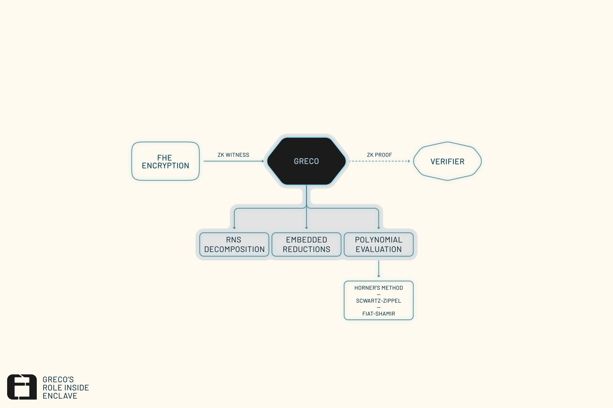
It achieves this by combining a few elegant ideas:

• RNS decomposition to split large ciphertext moduli into smaller, circuit-friendly parts.
• Embedded reductions that keep operations compatible with the SNARK field.
• Evaluation at a random point using the Schwartz–Zippel lemma and Fiat–Shamir heuristic to replace full polynomial checks with a single equality test.

The result is a lightweight, reusable component that connects ciphertexts and ZK proofs cleanly, and that can be plugged into many different FHE-based systems.

These guarantees matter in real multi-party encrypted systems. In Enclave, for example, E3s accept ciphertexts from many independent data providers who cannot see one another’s inputs but must still produce a correct joint result. GRECO ensures that each participant’s ciphertext matches the value they are proving about, so the encrypted execution that follows runs on data that is both private and consistent.

This post is part of our new Enclave Cryptography series. Subscribe below to get updates when we publish new entries, and join our Telegram if you’d like to discuss with or ask questions directly to the team.

Join Telegram